 Simulation Software for Fluids and Solids
Simulation H-Beam Stress Analysis
The simulation of an H-beam (stress analysis) in this case study is modeled as a linear elastic material in accordance with Hooke's law. The computation is performed as a static analysis based on the initial CAD geometry. A distributed load is applied to the upper side of the H-beam, resulting in the typical deformation pattern (see Figure 4 shown as superelevation).
Although a linear elastic material is used in this case study, NOGRID software is also capable of computing viscoelastic materials. In contrast to purely elastic bodies, a viscoelastic material has both elastic and viscous components. The viscosity of a viscoelastic material gives the body a strain-rate dependence over time. Purely elastic materials do not dissipate energy when a load is applied and subsequently removed. In contrast, a viscoelastic material dissipates energy under loading and unloading. Viscoelastic behavior has elastic and viscous components modeled as linear combinations of springs and dampers, respectively. Each model differs in the arrangement of these elements. The elastic components can be modeled as springs with elastic constant E, according to the formula:
σ = Eε
where σ is the stress, E is the elastic modulus of the material, and ε is the strain that occurs under the given stress, similar to Hooke's law. The viscous components can be modeled as dampers, so the relationship between stress and strain rate can be given as:
σ = η dε/dt
where σ is the stress, η is the viscosity of the material, and dε/dt is the time derivative of the strain.


The implemented Maxwell model is represented by a purely viscous damper and a purely elastic spring connected in series. According to this model, when the material subjected to a constant strain, the stress gradually relaxes. When a material is put under a constant stress, the strain has two components. First, an elastic component occurs instantaneously, corresponding to the spring, and relaxes immediately upon release of the stress. The second is a viscous component that grows with time as long as the stress is applied.
The implemented Kelvin–Voigt model consists of a Newtonian damper and a Hookean elastic spring connected in parallel. This model represents a solid undergoing reversible, viscoelastic strain. Upon application of a constant stress, the material deforms at a decreasing rate, asymptotically approaching the steady-state strain. When the stress is released, the material gradually relaxes to its undeformed state. Without viscous stress (η=0), the material is fully elastic, and only Hooke's law is valid.
In addition, the Generalized Maxwell model, also known as the Wiechert model, is implemented as well and it is the most general form of the linear model for viscoelasticity. It takes into account that the relaxation does not occur at a single time, but at a distribution of times. The Generalized Maxwell model consists of one or more Maxwell elements (viscous damper and elastic spring connected in series), an optional pure viscous, and an optional pure elastic element, all assembled in parallel. One special deduction of the Generalized Maxwell model implemented in NOGRID software is the Tool-Narayanaswamy-Moynihan model.
NOGRID points can be used for designing and problem solving for all kinds of stress related tasks.
Capabilities of NOGRID points CFD software
NOGRID combines the capability to handle stress computations for large deformations and a wide range of viscoelastic materials. It allows the simulation of any conceivable geometry and operating mode, such as
- fully 3D computation solving viscoelastic material behavior
- easy and intuitive setup
- freely definable material properties by user equations or user-defined curves
- Structure-Structure Interaction with viscoelastic materials
- Fluid-Structure Interaction using all implemented viscoelastic models
- computation of moving parts or moving boundaries in combination with viscoelastic materials
Why choose Nogrid?
NOGRID provides professional CFD software for the simulation of fluid flow, heat and mass transfer, and chemical reactions. Its efficient modelling workflow helps engineers analyse flow behaviour, evaluate designs and make informed decisions without creating a conventional volume mesh.
Faster model preparation
With NOGRID, only the geometry boundary needs to be meshed. The finite points inside the fluid domain are generated automatically according to user-defined settings, both at the start of the simulation and during the calculation.
This approach reduces preprocessing effort and makes it easier to prepare complex geometries and cavities for simulation.
Efficient CFD workflow
The modelling process follows four straightforward steps:
Build the geometry. Mesh the boundary. Define the simulation. Start the calculation.
NOGRID is designed to provide short computation times, including for applications involving complex cavities. Engineers can use the resulting data to examine flow distribution and other relevant flow characteristics.
Better insight into fluid-flow processes
CFD solves the fundamental equations governing fluid flow. NOGRID software enables engineers to predict and analyse the behaviour of fluids and related physical processes before or alongside physical testing.
The simulation results can support:
- evaluation and comparison of design alternatives
- optimisation of construction and operating parameters
- improved planning reliability
- reduction of development time and testing effort
- faster progression from design to market or operation
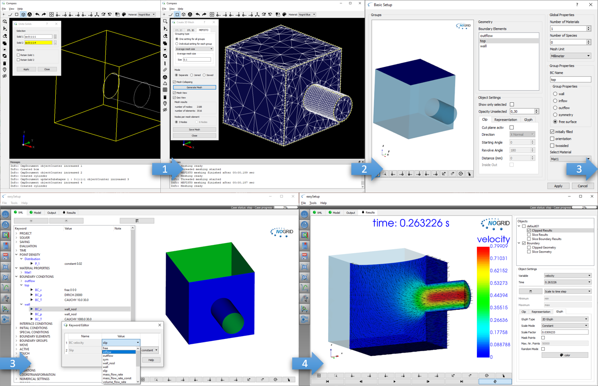
Steps from geometry generation to simulation results
TRAINING
Our two-day training courses teach participants how to set up, run and evaluate simulations efficiently with NOGRID CFD software. The courses include practical guidance for handling different types of simulation cases.
For more details please refer to Training Courses →
Technical Support
Professional support is available from the beginning of your work with NOGRID. Our technical team assists users by telephone and email with software operation, case setup and simulation-related questions.
For more details please refer to Software Support →
Simulation Service
When internal time, expertise or resources are limited, NOGRID can support your project with individual numerical simulation services. Our engineers develop and evaluate CFD models based on the specific requirements of your application.
For more details please refer to Software Support →